Categorising Geographic Data with Alteryx

Introduction

Latitude and longitude values are essential for mapping in a data visualisation. However, they are less useful for other visualisations, such as bar charts where categorical data is used. Categorising geographic data can be tedious, but Alteryx can automate the process in just a few steps. This article demonstrates a method of categorising latitude and longitude values using publically available .shp files.

Step 1: Obtain Digital Boundary Files

In this example, we will convert latitude and longitude values into Australian states using publicly available digital boundary files from the Australian Bureau of Statistics (ABS)

Download the States and Territories – 2021 – Shapefile and unzip it into your project folder. The archive contains several files, however only the .shp file is required.

Step 2: Load Geographic Data

Geographic data (latitude and longitude values) can be loaded from a .csv file using the Input Data tool. To simplify the next steps, rename the latitude and longitude fields if they have other names. Additionally, check for any issues in the latitude and longitude values. For instance, some rows in this data contain invalid values (see record 3 below), which will be replaced with nulls using the Formula tool.

Use the Create Points tool to convert latitude and longitude values into spatial coordinates by selecting longitude as the X Field and latitude as the Y Field.

Step 3: Load Digital Boundaries

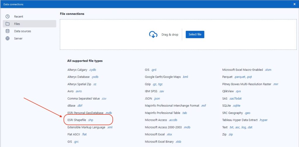
Use the Input Data tool to load the .shp file, selecting the ESRI Shapefile (.shp) option when setting up the connection.

Once loaded, the data should resemble the example below.

For this example, the fields used are STE_NAME21 and SpatialObj. STE_NAME21 contains the state names for the categories, while SpatialObj holds the digital boundaries for comparing geographic data.

Step 4: Categorise using Spatial Matching

Connect the output from the Create Points tool to the Targets (T) input of the Spatial Match tool. Connect the digital boundaries loaded in Step 3 to the Universe (U) input of the Spatial Match tool.

For the Targets Spatial Object Field, select ‘Centroid’ from the dropdown. For the Universe Spatial Object Field, select ‘SpatialObj’ from the dropdown.

The Spatial Match tool also functions as a Select tool, allowing you to choose specific fields for output and modify field names or data types as needed.

The Matched (M) output contains all matches, while the Unmatched (U) output includes any non-matches.

Once matched, the State Name column (renamed from STE_NAME21) can be used to categorise geographic data.

The final workflow is shown below. In this example, approximately 14% of the records could not be matched to a state. It is recommended to review the U output tag to ensure the results meet expectations.

Conclusion

This method simplifies the categorisation of geographic data, enhancing the scope of your analysis. By leveraging publicly available spatial data and Alteryx’s spatial tools, you can incorporate deeper location-based insights into your work.